Vector Databases: from Embedding to Applications

이 글은 Vector Databases: from Embedding to Applications 코스를 보고 정리한 글입니다.

---

Outline:

• How to obtain vector representations of data?
  • Embedding
• Searching for Similar Vectos
  • Distance Metrics
• Approximate Nearest Neighbors
  • ANN - Trade recall for accuracy
  • HNSW
• Vector DB's
  • CRUD Operations
  • Objects + Vectors
  • Inverted index - filtered search
• Sparse vs Dense Search
  • ANN search over Dense embeddings
  • Sparse Search
  • Hybrid Search
• Applications at Vector DBs in Industry

 

 

1. How to obtain vector representations of data

Embedding 의 정의:

• 컴퓨터가 우리의 데이터들 이미지나 텍스트와 같은 데이터를 이해하는 방법이다. 임베딩을 하면 데이터는 Vector 의 형식으로 표현되는데 이런 표현을 바탕으로 컴퓨터는 이해한다.
• 이렇게 표현하면 유사한 데이터는 유사한 벡터를 가지고도록 표현하게 되면서 이해하게 됨.

 

 

Vector 를 계산하는 방법을 4가지가 있다:

• Euclidean Distance(L2)
• Manhattan Distance(L1)
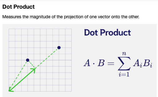
• Dot Product
• Cosine Distance

 

Euclidean Distance(L2) 를 계산하는 코드:

• 두 벡터 간의 직선 거리를 측정하는 방법임.
• 벡터간의 실제 물리적 거리를 비교할 때 사용되는 방법임.
• 데이터가 밀집되어있고, 모든 차원이 동일한 중요도를 가질 때 효과적임.

# Euclidean Distance
L2 = [(zero_A[i] - zero_B[i])**2 for i in range(len(zero_A))]
L2 = np.sqrt(np.array(L2).sum())
print(L2)

#An alternative way of doing this
np.linalg.norm((zero_A - zero_B), ord=2)

#Calculate L2 distances
print("Distance zeroA-zeroB:", np.linalg.norm((zero_A - zero_B), ord=2))
print("Distance zeroA-one:  ", np.linalg.norm((zero_A - one), ord=2))
print("Distance zeroB-one:  ", np.linalg.norm((zero_B - one), ord=2))

 

 

Manhattan Distance(L1) 를 계산하는 코드:

• 두 벡터 간의 각 차원의 절대 차이의 합을 계산하는 방법.
• 계산 방식은 각 차원의 차이의 절댓값을 모두더하는 것.
• 데이터의 각 차원이 독립적이고 차원 간의 차이가 중요한 경우 효과적임.

# Manhattan Distance
L1 = [zero_A[i] - zero_B[i] for i in range(len(zero_A))]
L1 = np.abs(L1).sum()

#an alternative way of doing this is
np.linalg.norm((zero_A - zero_B), ord=1)

#Calculate L1 distances
print("Distance zeroA-zeroB:", np.linalg.norm((zero_A - zero_B), ord=1))
print("Distance zeroA-one:  ", np.linalg.norm((zero_A - one), ord=1))
print("Distance zeroB-one:  ", np.linalg.norm((zero_B - one), ord=1))

 

 

Dot Product 를 계산하는 코드:

• 벡터 곱의 합을 계산하는 것.
• 벡터간의 유사성을 측정할 때 사용한다. 값이 클수록 두 벡터가 유사함을 나타냄.

# Dot Product
np.dot(zero_A,zero_B)

#Calculate Dot products
print("Distance zeroA-zeroB:", np.dot(zero_A, zero_B))
print("Distance zeroA-one:  ", np.dot(zero_A, one))
print("Distance zeroB-one:  ", np.dot(zero_B, one))

 

 

Cosine Distance 를 계산하는 코드:

• 벡터간의 각도를 측정하는 방법
• 벡터의 크기보다 방향에 더 집중한다. 이것도 유사도를 측정할 때 자주 사용함.

# Cosine Distance
cosine = 1 - np.dot(zero_A,zero_B)/(np.linalg.norm(zero_A)*np.linalg.norm(zero_B))
print(f"{cosine:.6f}")

# Cosine Distance function
def cosine_distance(vec1,vec2):
  cosine = 1 - (np.dot(vec1, vec2)/(np.linalg.norm(vec1)*np.linalg.norm(vec2)))
  return cosine

#Cosine Distance
print(f"Distance zeroA-zeroB: {cosine_distance(zero_A, zero_B): .6f}")
print(f"Distance zeroA-one:   {cosine_distance(zero_A, one): .6f}")
print(f"Distance zeroB-one:   {cosine_distance(zero_B, one): .6f}")

 

 

실제 임베딩을 이용해서 거리를 계산하는 코드:

# - embedding0 - 'The team enjoyed the hike through the meadow'
# - embedding1 - The national park had great views'
# - embedding2 - 'Olive oil drizzled over pizza tastes delicious'

#Dot Product
print("Distance 0-1:", np.dot(embedding[0], embedding[1]))
print("Distance 0-2:", np.dot(embedding[0], embedding[2]))
print("Distance 1-2:", np.dot(embedding[1], embedding[2]))

#Cosine Distance
print("Distance 0-1: ", cosine_distance(embedding[0], embedding[1]))
print("Distance 0-2: ", cosine_distance(embedding[0], embedding[2]))
print("Distance 1-2: ", cosine_distance(embedding[1], embedding[2]))

 

 

Q) 왜 자연어 처리에서는 Dot Prodct 와 Cosine Distance 를 주로 이용하는건가?

 

두 방식이 유사도 계산이라서.

 

 

2. Searching for Similar Vectos

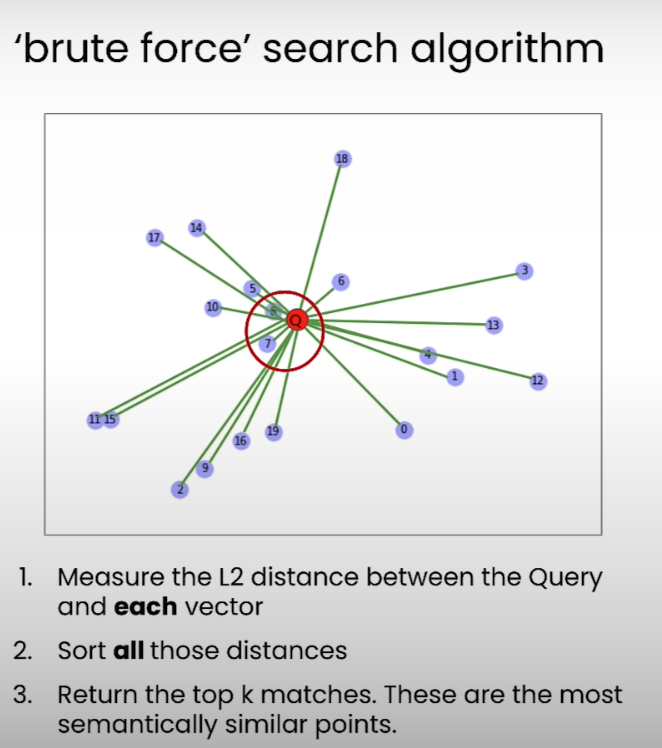
Brute-force KNN 방식과 단점:

• 3가지 Step 을 이용해서 해당 벡터와 가까운 벡터를 검색한다:
  • 유클리드 거리 검색 (L2) 를 이용해서 주어진 쿼리 벡터와 데이터 포인트들의 모든 거리를 계산한다.
  • 거리가 낮은 순으로 정렬한다
  • Top K 개 만큼을 뽑는다.
• 이 방식은 간단하고 직관적이긴 하나, 대규모 데이터 셋에는 적합하지 않음. 벡터의 차원이 증가될수록, 데이터 포인트가 커질수록 거리 계산 비용은 점점 더 늘어난다. 확장성 있는 방법은 아님.

 

 

3. Approximate nearest neighbours

이전에 배운 Brute-force KNN 알고리즘의 단점인 Scalibility 를 해결할 수 있는 방법으로 ANN 이 있음.

 

여기서는 대표적인 ANN 알고리즘으로 HNSW (Hierarchical Navigable Small World) 에 대해 배워볼거임.

 

HNSW 는 NSW(Navigable Small World) 에서 Layer 개념을 추가한 것으로 NSW 부터 알아보자.

 

NSW 는 소셜 네트워크에서 영감을 받은 알고리즘임. 내가 6명의 친구 다리만 건너면 전세계의 모든 사람들과 연결될 수 있다는 논리로 이뤄진 것.

 

NSW 의 Constructing 단계 부터 살펴보자.

• 8개의 벡터로 시작하며, 0번부터 하나씩 그래프를 만든다.

 

 

• 1번 노드가 추가되고 가장 가까운 2개의 노드 중 하나인 0번 노드와 연결된다. 그리고 2번 노드가 들어오는 상황임.

 

 

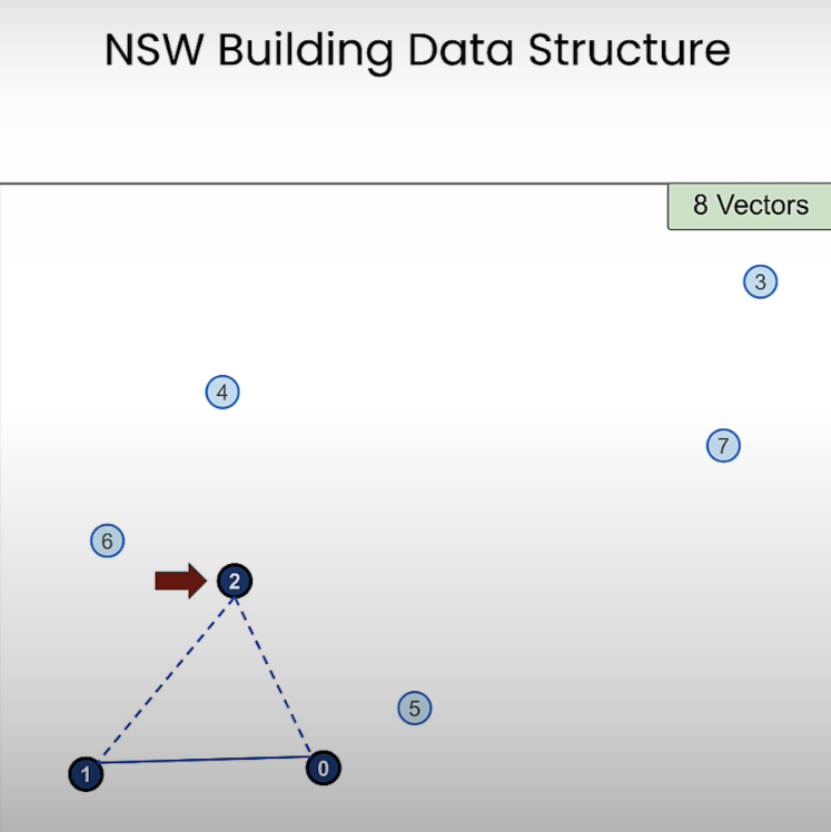
• 2번 노드도 가장 가까운 노드인 0과 1번 노드와 연결되고 이제 3번 노드도 들어온다. 3번 노드 또한 가장 가까운 2개의 노드인 0과 2번 노드와 연결되고, 4번 노드가 들어오는 상황임

 

 

• 이런식으로 노드가 연결되면 최종적으로는 이것과 같을 것. 지금은 노드당 2개의 Edge 만 있는데 실제로 사용할 때는 이 변수도 튜닝해야함. 32개 정도를 쓴다고 한다.

 

 

이제 NSW 의 Searching 단계를 시작해보자. 시작은 임의의 노드부터 시작한다.

 

 

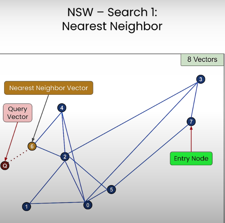
• 노드 5번이 쿼리 벡터 노드와 더 가까우니까 7번 노드에서 5번 노드로 이동한다.

 

 

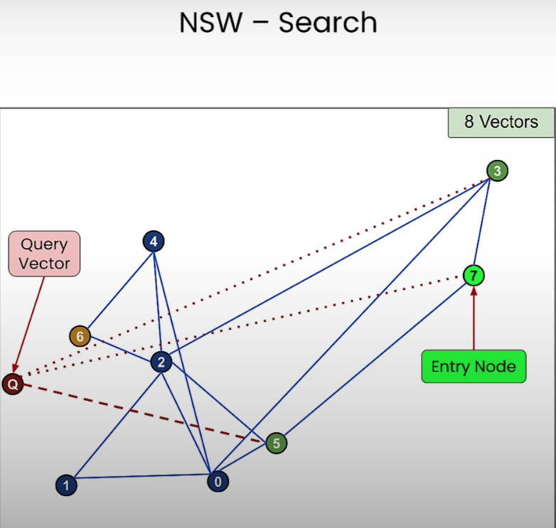
• 그리고 5번 노드와 연결된 0번과 2번 노드 중 쿼리 벡터와 더 가까운 노드인 2번 노드로 이동하게 된다.

 

 

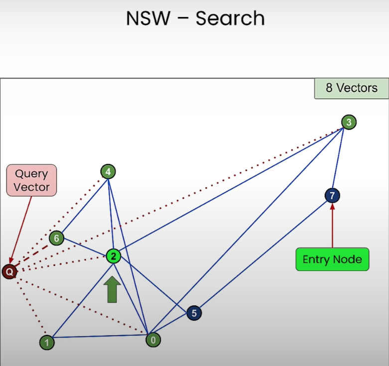
• 이런식으로 검색을 하다보면 쿼리 벡터 노드와 가장 가까운 6번 노드가 검색되게 된다. 6번 노드와 연결된 노드 중에 쿼리 벡터 노드와 더 가까운 노드가 없기 때문임.

 

 

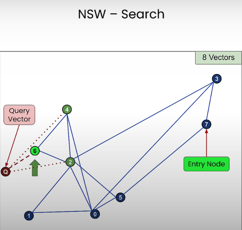
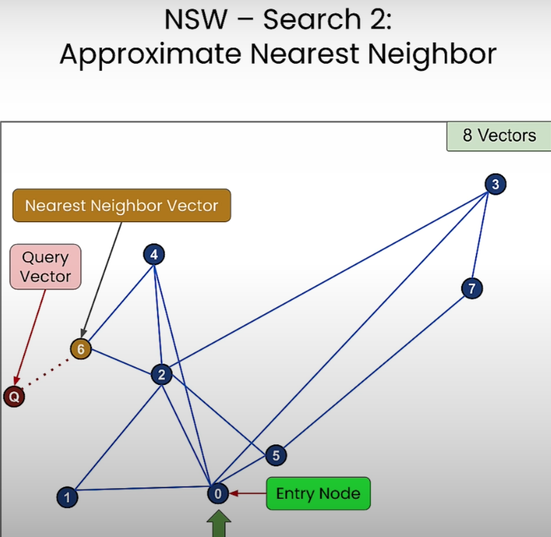
이런 NSW 방식은 항상 정확한 검색을 제공하지 않는다. Entry Node 의 시작 지점에 따라서 연결된 그래프 노드들 중에 쿼리 벡터와 가장 가까운 노드로 탐색하게 되지만 이게 항상 최적값을 보장하지는 않음.

 

 

HNSW 는 여기에다가 Layer 를 추가한 방식이다. 가장 최상위 레이어부터 최하위 레이어까지 검색을 하는 방법임.

• 레이어 내에서 검색하는 방법은 NSW 와 동일하다.

 

 

HNSW 에서 노드를 레이어에 할당하는 방법은 무작위다. 그러나 상위 레이어에 할당될 확률은 하위 레이어보다 지수적으로 작다. 그래서 최하위 레이어가 가장 많이 할당됨.

 

그리고 HNSW 에서는 상위 레이어의 노드는 하위 레이어에도 존재한다. 중첩되어 있다고 알면 됨. 즉 최상위 레이어에 속한 노드는 모든 하위 레이어에도 속함.

 

이렇게 중첩되어 있기 때문에 상위 레이어에서의 탐색은 하위 레이어로 이어진다.

 

HNSW 의 시간 복잡도는 상위 레이어에서 시작해서 하위 레이어로 내려가는 계층적 탐색을 수행하고, 각 레이어의 노드 수는 지수적으로 감소하므로, 레이어의 탐색은 LogN 에 비례한다.

 

그리고 각 레이어에서 쿼리 벡터와 가장 가까운 노드를 탐색하는 과정은 ef 파라미터에 의해 조정될 수 있음. ef 파라미터가 클수록 더 많은 노드를 탐색하므로 정확도가 높아진다. 대신 성능은 낮아짐.

 

Webviate 를 이용한 Pure Vector Search 를 검색하는 코드:

import weaviate, json
from weaviate import EmbeddedOptions

client = weaviate.Client(
    embedded_options=EmbeddedOptions(),
)

client.is_ready()

# resetting the schema. CAUTION: This will delete your collection 
# if client.schema.exists("MyCollection"):
#     client.schema.delete_class("MyCollection")

schema = {
    "class": "MyCollection",
    "vectorizer": "none",
    "vectorIndexConfig": {
        "distance": "cosine" # let's use cosine distance
    },
}

client.schema.create_class(schema)

print("Successfully created the schema.")

data = [
   {
      "title": "First Object",
      "foo": 99, 
      "vector": [0.1, 0.1, 0.1, 0.1, 0.1, 0.1]
   },
   {
      "title": "Second Object",
      "foo": 77, 
      "vector": [0.2, 0.3, 0.4, 0.5, 0.6, 0.7]
   },
   {
      "title": "Third Object",
      "foo": 55, 
      "vector": [0.3, 0.1, -0.1, -0.3, -0.5, -0.7]
   },
   {
      "title": "Fourth Object",
      "foo": 33, 
      "vector": [0.4, 0.41, 0.42, 0.43, 0.44, 0.45]
   },
   {
      "title": "Fifth Object",
      "foo": 11,
      "vector": [0.5, 0.5, 0, 0, 0, 0]
   },
]

client.batch.configure(batch_size=10)  # Configure batch

# Batch import all objects
# yes batch is an overkill for 5 objects, but it is recommended for large volumes of data
with client.batch as batch:
  for item in data:

      properties = {
         "title": item["title"],
         "foo": item["foo"],
      }

      # the call that performs data insert
      client.batch.add_data_object(
         class_name="MyCollection",
         data_object=properties,
         vector=item["vector"] # your vector embeddings go here
      )

# Check number of objects
response = (
    client.query
    .aggregate("MyCollection")
    .with_meta_count()
    .do()
)

print(response)


response = (
    client.query
    .get("MyCollection", ["title"])
    .with_near_vector({
        "vector": [-0.012, 0.021, -0.23, -0.42, 0.5, 0.5]
    })
    .with_limit(2) # limit the output to only 2
    .do()
)

result = response["data"]["Get"]["MyCollection"]
print(json.dumps(result, indent=2))


response = (
    client.query
    .get("MyCollection", ["title"])
    .with_near_vector({
        "vector": [-0.012, 0.021, -0.23, -0.42, 0.5, 0.5]
    })
    .with_limit(2) # limit the output to only 2
    .with_additional(["distance", "vector, id"])
    .do()
)

result = response["data"]["Get"]["MyCollection"]
print(json.dumps(result, indent=2))


response = (
    client.query
    .get("MyCollection", ["title", "foo"])
    .with_near_vector({
        "vector": [-0.012, 0.021, -0.23, -0.42, 0.5, 0.5]
    })
    .with_additional(["distance, id"]) # output the distance of the query vector to the objects in the database
    .with_where({
        "path": ["foo"],
        "operator": "GreaterThan",
        "valueNumber": 44
    })
    .with_limit(2) # limit the output to only 2
    .do()
)

result = response["data"]["Get"]["MyCollection"]
print(json.dumps(result, indent=2))

response = (
    client.query
    .get("MyCollection", ["title"])
    .with_near_object({ # the id of the the search object
        "id": result[0]['_additional']['id']
    })
    .with_limit(3)
    .with_additional(["distance", "id"])
    .do()
)

result = response["data"]["Get"]["MyCollection"]
print(json.dumps(result, indent=2))

 

 

4. Vector Database

여기서는 Weaviate 라는 Vector Database 를 이용해서 CRUD 연산등을 하는 방법에 대해 알아보자.

1. 먼저 Sample Data 다운로드 하는 코드:

import requests
import json

# Download the data
resp = requests.get('https://raw.githubusercontent.com/weaviate-tutorials/quickstart/main/data/jeopardy_tiny.json')
data = json.loads(resp.text)  # Load data

# Parse the JSON and preview it
print(type(data), len(data))

def json_print(data):
    print(json.dumps(data, indent=2))

json_print(data[0])

 

 

2. Weaviate Client 를 만드는 코드

import weaviate, os
from weaviate import EmbeddedOptions
import openai

from dotenv import load_dotenv, find_dotenv
_ = load_dotenv(find_dotenv()) # read local .env file
openai.api_key = os.environ['OPENAI_API_KEY']

client = weaviate.Client(
    embedded_options=EmbeddedOptions(),
    additional_headers={
        "X-OpenAI-BaseURL": os.environ['OPENAI_API_BASE'],
        "X-OpenAI-Api-Key": openai.api_key  # Replace this with your actual key
    }
)
print(f"Client created? {client.is_ready()}")

 

 

3. Collection 을 만드는 코드. Collection 은 MongoDB 의 Collection 이라고 생각하면 됨.

• vectorizer 에서 text2vec-openai 를 입력했는데 이러면 임베딩 벡터를 생성하는 역할을 하는 모델로 OpenAI 에서 지원해주는 text2vec-openai 모델이 알아서 잘 만들어줌.

# resetting the schema. CAUTION: This will delete your collection 
if client.schema.exists("Question"):
    client.schema.delete_class("Question")
class_obj = {
    "class": "Question",
    "vectorizer": "text2vec-openai",  # Use OpenAI as the vectorizer
    "moduleConfig": {
        "text2vec-openai": {
            "model": "ada",
            "modelVersion": "002",
            "type": "text",
            "baseURL": os.environ["OPENAI_API_BASE"]
        }
    }
}

client.schema.create_class(class_obj)

 

 

4. 데이터들을 이제 Vector Database 에 적재.

with client.batch.configure(batch_size=5) as batch:
    for i, d in enumerate(data):  # Batch import data

        print(f"importing question: {i+1}")

        properties = {
            "answer": d["Answer"],
            "question": d["Question"],
            "category": d["Category"],
        }

        batch.add_data_object(
            data_object=properties,
            class_name="Question"
        )

 

 

데이터의 표현은 아래와 같을거임

{
  "Category": "SCIENCE",
  "Question": "This organ removes excess glucose from the blood & stores it as glycogen",
  "Answer": "Liver"
}

 

 

데이터가 잘 들어갔는지 보고 싶다면 아래의 코드를 실행해보면 됨.

count = client.query.aggregate("Question").with_meta_count().do()
json_print(count)

 

 

5. 실제 검색을 해보는 쿼리 코드

response = (
    client.query
    .get("Question",["question","answer","category"])
    .with_near_text({"concepts": "biology"})
    .with_additional('distance')
    .with_limit(2)
    .do()
)

json_print(response)

 

 

5-1 실제 검색을 하는데 threhold 를 지정해서 검색하는 코드

response = (
    client.query
    .get("Question", ["question", "answer"])
    .with_near_text({"concepts": ["animals"], "distance": 0.24})
    .with_limit(10)
    .with_additional(["distance"])
    .do()
)

json_print(response)

 

 

6. CRUD 하는 코드:

#Create an object
object_uuid = client.data_object.create(
    data_object={
        'question':"Leonardo da Vinci was born in this country.",
        'answer': "Italy",
        'category': "Culture"
    },
    class_name="Question"
 )

# Read 
data_object = client.data_object.get_by_id(object_uuid, class_name="Question")
json_print(data_object)

data_object = client.data_object.get_by_id(
    object_uuid,
    class_name='Question',
    with_vector=True
)

json_print(data_object)

# Update 
client.data_object.update(
    uuid=object_uuid,
    class_name="Question",
    data_object={
        'answer':"Florence, Italy"
    })

# Delete 
data_object = client.data_object.get_by_id(
    object_uuid,
    class_name='Question',
)

json_print(data_object)

 

 

5. Sparse, Dense, and Hybrid Search

Dense Search 는 우리가 알고 있는 Embedding Vector 를 이용한 Semantic Search 를 말하고, Sparse Search 는 쿼리 벡터에 포함되어 있는 단어를 가지고 매칭된게 있는지 확인해서 검색하는 전통적인 검색 방법을 말한다.

 

Dense Search 는 여러 한계점도 있기 때문에 Spare Search 와 같이 섞어서 이용하는 Hybrid Search 라는 개념도 나옴.

 

Dense Search 의 한계점:

• 임베딩 모델의 언어 영억에 의존적이다. 특정 도메인 (e.g 의료, 법률) 과 관련되서 유사도 검색을 하려고 하는데 언어 모댈이 그 도메인에서 나오는 단어들에 대한 감각이 없다면 유사도 검색은 잘 이뤄지지 않음.
• 반대로 임베딩 모델이 특정 도메인에 최적화되어 있다면 제너럴한 질문에 대해서 유사도 검색을 잘 하지 못하는 문제가 발생함.
• 임베딩 모델은 제품의 Serial Number (e.g BBBB309940 등) 에 대해서 의미에 대한 유사도 검색을 수행하려고 해서 의도하지 않은 결과 문서가 반환될 수도 있음.

 

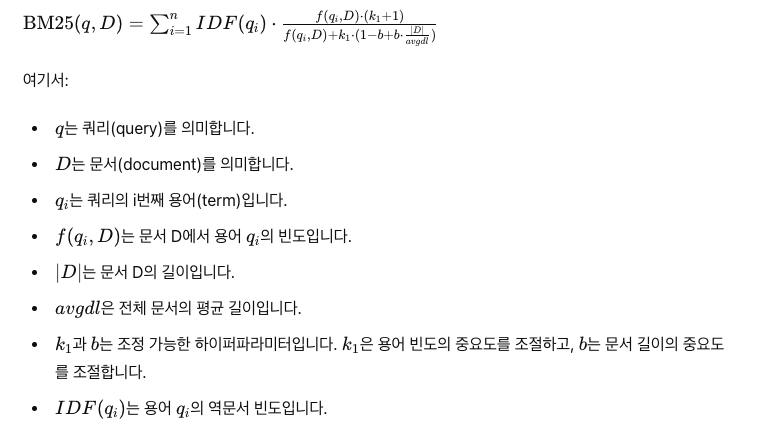
대표적인 Spare Search 기법인 BM25

• 공식은 아래와 같지만 알아야 할 건 다음과 같다:
• 역 문서 빈도 (IDF): 드물게 등장하는 단어가 중요한 단어라고 판단해서 높은 가중치를 부여해서 스코어링을 한다.
• 용어 빈도 (TF): IDF 와 반대로 문서 내에서 자주 등장하는 단어가 그 문서 내에서 중요한 단어라고 판단해서 스코어링을 높임.
• 문서 길이 보정: 문서 길이가 길어질수록 단어 출현 빈도수를 고려한다. 문서 길이가 길수록 자주 등장하는 단어는 가중치를 적게 줌.
• 이렇게 3가지 기준을 종합해서 스코어링을 매기는 기법임.

 

Hybrid Search 는 Dense Search 의 스코어 점수와 Sparse Search 의 스코어 점수를 합쳐서 랭킹을 매겨서 검색하는 방법이다.

 

Webviate 를 이용해서 Hybrid Search 를 하는 예시를 보자.

 

먼저 Webviate 인스턴스를 생성하고, 데이터를 적재하는 코드는 다음과 같다.

import requests
import json

# Download the data
resp = requests.get('https://raw.githubusercontent.com/weaviate-tutorials/quickstart/main/data/jeopardy_tiny.json')
data = json.loads(resp.text)  # Load data

# Parse the JSON and preview it
print(type(data), len(data))

def json_print(data):
    print(json.dumps(data, indent=2))

import weaviate, os
from weaviate import EmbeddedOptions
import openai

from dotenv import load_dotenv, find_dotenv
_ = load_dotenv(find_dotenv()) # read local .env file
openai.api_key = os.environ['OPENAI_API_KEY']

client = weaviate.Client(
    embedded_options=EmbeddedOptions(),
    additional_headers={
        "X-OpenAI-Api-BaseURL": os.environ['OPENAI_API_BASE'],
        "X-OpenAI-Api-Key": openai.api_key,  # Replace this with your actual key
    }
)
print(f"Client created? {client.is_ready()}")

# Uncomment the following two lines if you want to run this block for a second time.
if client.schema.exists("Question"):
   client.schema.delete_class("Question")

class_obj = {
    "class": "Question",
    "vectorizer": "text2vec-openai",  # Use OpenAI as the vectorizer
    "moduleConfig": {
        "text2vec-openai": {
            "model": "ada",
            "modelVersion": "002",
            "type": "text",
            "baseURL": os.environ["OPENAI_API_BASE"]
        }
    }
}

client.schema.create_class(class_obj)

with client.batch.configure(batch_size=5) as batch:
    for i, d in enumerate(data):  # Batch import data

        print(f"importing question: {i+1}")

        properties = {
            "answer": d["Answer"],
            "question": d["Question"],
            "category": d["Category"],
        }

        batch.add_data_object(
            data_object=properties,
            class_name="Question"
        )

 

 

Webviate 를 이용해 Dense Search 를 하는 코드 예시는 다음과 같다:

response = (
    client.query
    .get("Question", ["question", "answer"])
    .with_near_text({"concepts":["animal"]})
    .with_limit(3)
    .do()
)

json_print(response)

 

 

Webviate 를 이용해 Sparse Search 를 하는 코드 예시는 다음과 같다:

response = (
    client.query
    .get("Question",["question","answer"])
    .with_bm25(query="animal")
    .with_limit(3)
    .do()
)

json_print(response)

 

 

Webviate 를 이용해 Hybrid Search 를 하는 코드 예시는 다음과 같다:

• 여기서 중요한 파라미터인 alpha 가 나온다. alpha 가 1에 가까울수록 Vector Search 에 높은 가중치를 주게되고, 0에 가까울수록 Sparse Search 에 높은 가중치를 주게 된다.
• 즉 1을 주면 Dense Search 만 쓰게되고, 0을 주게되면 Sparse Search 를 쓰게됨.

response = (
    client.query
    .get("Question",["question","answer"])
    .with_hybrid(query="animal", alpha=0.5)
    .with_limit(3)
    .do()
)

json_print(response)

 

 

6. Application - Multilingual Search

Multilingual Search 란?

• 같은 임베딩 된 문서라도 다양한 언어로 검색할 수 있는 걸 말한다. 이렇게 되려면 임베딩 모델이 다국어 능력에 강해야함. 일반적으로 같은 내용이더라도 한국어로 되어있느냐, 영어로 되어있느냐에 따라서 임베딩 벡터가 다르다. 그러나 다국어 훈련이 된 임베딩 모델이 벡터를 생성한다면 비슷하게 나올거임.

 

여기서는 Webviate 를 이용해서 Multilingual Search 를 해서 RAG 를 구현하는 코드 예시를 보여줌

 

먼저 Webviate 클라이언트 인스턴스 생성과 데이터 적재:

• COHERE_API_KEY 는 Multilingual Search 를 위해서 사용하기 위한 키임. Webviate 클라우드를 이용해서 사용

def json_print(data):
    print(json.dumps(data, indent=2))

import weaviate, os, json
import openai
from dotenv import load_dotenv, find_dotenv
_ = load_dotenv(find_dotenv()) # read local .env file

auth_config = weaviate.auth.AuthApiKey(api_key=os.getenv("WEAVIATE_API_KEY"))

client = weaviate.Client(
    url=os.getenv("WEAVIATE_API_URL"),
    auth_client_secret=auth_config,
    additional_headers={
        "X-Cohere-Api-Key": os.getenv("COHERE_API_KEY"),
        "X-Cohere-BaseURL": os.getenv("CO_API_URL")
    }
)

client.is_ready() #check if True

 

 

그냥 검색을 하면 다양한 언어로 작성된 위키 피디아 문서가 검색됨:

response = (client.query
            .get("Wikipedia",['text','title','url','views','lang'])
            .with_near_text({"concepts": "Vacation spots in california"})
            .with_limit(5)
            .do()
           )

json_print(response)

 

 

영어로 작성된 문서만 검색되도록 필터 조건을 넣을수도 있다.

response = (client.query
            .get("Wikipedia",['text','title','url','views','lang'])
            .with_near_text({"concepts": "Vacation spots in california"})
            .with_where({
                "path" : ['lang'],
                "operator" : "Equal",
                "valueString":'en'
            })
            .with_limit(3)
            .do()
           )

json_print(response)

 

 

영어로 작성된 문서만 검색하지만 다른 외국어로 질문을 할 수도 있음:

response = (client.query
            .get("Wikipedia",['text','title','url','views','lang'])
            .with_near_text({"concepts": "Miejsca na wakacje w Kalifornii"})
            .with_where({
                "path" : ['lang'],
                "operator" : "Equal",
                "valueString":'en'
            })
            .with_limit(3)
            .do()
           )

json_print(response)

 

 

간단하게 Webviate 를 이용해서 Vector Database 에거 검색한 내용을 바탕으로 RAG 를 구현하는 코드:

prompt = "Write me a facebook ad about {title} using information inside {text}"
result = (
  client.query
  .get("Wikipedia", ["title","text"])
  .with_generate(single_prompt=prompt)
  .with_near_text({
    "concepts": ["Vacation spots in california"]
  })
  .with_limit(3)
).do()

json_print(result)

 

 

Vector Store 에서 검색한 내용을 모두 한방에 프롬포트에 넣어서 사용하는 RAG 구현 코드:

generate_prompt = "Summarize what these posts are about in two paragraphs."

result = (
  client.query
  .get("Wikipedia", ["title","text"])
  .with_generate(grouped_task=generate_prompt) # Pass in all objects at once
  .with_near_text({
    "concepts": ["Vacation spots in california"]
  })
  .with_limit(3)
).do()

json_print(result)